The Similarity Analysis for Documents can be used to check the similarity or dissimilarity of various documents in terms of code occurrence and code frequency. The values of document variables can also be included.
Starting the Similarity Analysis
- Activate all documents you would like to include in the Similarity Analysis.
- It is also helpful to activate all codes you wish to use for determining similarity.
- From the Mixed Methods menu tab, click
 Similarity Analysis for Documents. A window will appear that contains all previously created similarity and distance matrices.
 - Click on the
 New Similarity/Distance matrix symbol to begin the similarity analysis.
Setting the parameters for the analysis
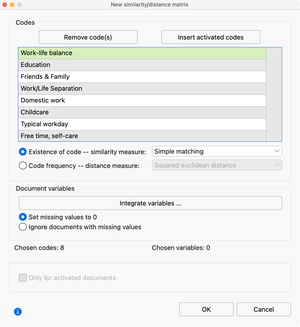
A dialog window will appear in which you can select the codes and variables and specify the type of analysis.

In the upper section, you can add the codes you wish to include in the analysis. You can add all activated codes directly via the Paste activated codes button.
Next, select the type of analysis:
Existence of code – Generates a similarity matrix that considers only whether the selected codes occur in the document or not.
Code frequency – Generates a distance matrix that takes the distance of individual codes into consideration.
Similarity measures with the option “Existence of code”
To calculate similarity, various options are available. All of the calculations are based on a four-field table of the following type that is generated for each paired combination of documents (in the background, not displayed):
| Document A | |||
| Code/Variable value exists | Code/Variable value does not exist | ||
| Document B | Code/Variable value exists | a | b |
| Code/Variable value does not exist | c | d | |
a = Number of codes or variable values that are identical in both documents.
d = Number of codes or variable values that do not exist in both documents.
b and c = Number of codes or variable values that exist in only one document.
The calculation options differ in, among other things, the extent to which field "d", the non-existence in both documents, is considered a match.
Simple match = (a + d) / (a + b + c + d) – Both existence and non-existence are counted as a match. The result is the percentage match.
Jaccard = a / (a + b + c) – Non-existence is completely ignored.
Kuckartz & Rädiker zeta = (2a + d) / (2a + b + c + d) – Existence is counted twice, non-existence once.
Russel & Rao = a / (a + b + c + d) – Only existence is considered a match, but non-existence reduces the similarity.
Distance measures with the option “Code frequency”
To calculate the distance between two documents based on “Code frequency”, the following options are available in which the code frequencies of two documents will be compared:
Squared euclidean distance = The sum of squared deviations (higher deviations will be rated higher as lower ones because of squaring the deviations).
Block distance = The sum of absolute deviations.
Including variables
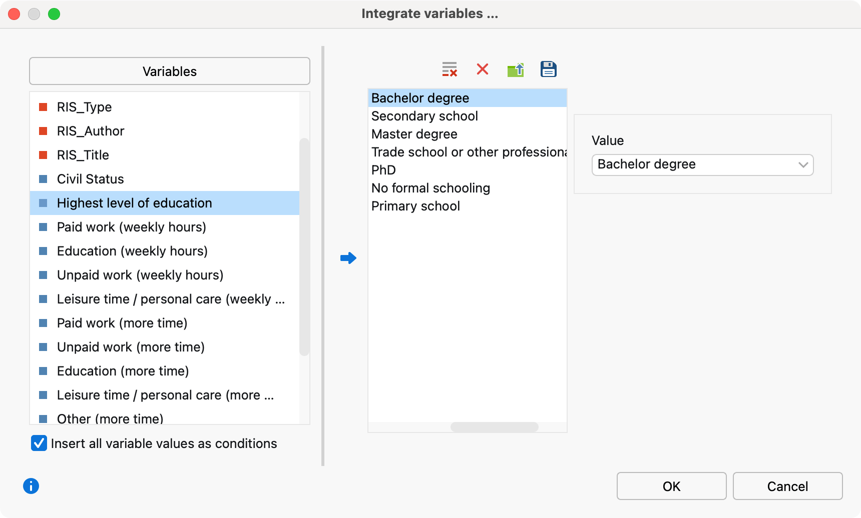
If you want to include variables in addition to codes in the similarity analysis, click the Integrate variables button. If you selected “Existence of code” as the type of analysis, you can then select which variable values MAXQDA should evaluate in the dialog window. If the selected variable value exists in both documents, this is evaluated as a match (type “a” in the table above). In the dialog window, only variables of type “Text”, “Boolean (true/false)”, “Date” as well as categorical “Integer” and categorical “Decimal” are listed.

If you selected "Code frequency" as the type of analysis, another dialog window will appear that contains only integer or floating-point variables, that are not marked as "categorical".
Dealing with missing variable values
You can choose how missing values are handled:
Set missing values to 0 – IIf a variable value does not exist, it is set to 0 (which equals the average due to the z- standardization). Using this option, documents with missing values are included in the analysis.
Ignore documents with missing values – If in a document one value of the selected variables is missing, the entire document will be ignored in the analysis.
The final similarity or distance matrix
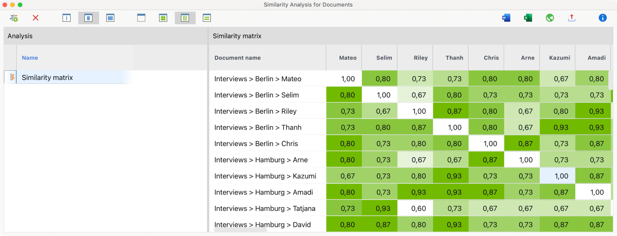
The following figure shows a similarity matrix for five interviews. The selected documents are listed both in the rows and in the columns:

The default shadowed color helps to interpret the cells, which in a similarity matrix can have a value of 0 (no similarity) to 1 (identical): The darker the green, the more similar the two documents are in terms of the selected code and variable values. In the figure, for example, you can see that "Sam" completely coincides with "Jamie" both in their codes and their variable values.
The matrix is sortable: click on a column header to sort the documents in the rows according to their similarity to the clicked document.
The Similarity Analysis toolbar
In addition to the usual export options, the following functions can be accessed from the toolbar:
New similarity/distance matrix – Calls up the dialog window where you can create a new matrix.
Delete – Deletes the selected matrix.
Names, columns: none, short, full – Controls column width.
No color highlight – Turns off green highlighting.
Color highlight refers to whole matrix – The highlight color takes into account the values of all cells. The same values will have the same highlight color in the table.
Color highlight refers to columns – In each column, the colors are graduated from white to green. In this way, you can see at a glance which documents are particularly similar to the document in the column. The same values in the matrix may be colored differently.
Color highlight refers to rows – In each row, the colors are graduated from white to green. In this way, you can see at a glance which documents are particularly similar to the document in the row. The same values in the matrix may be colored differently.
Distance matrices look identical to similarity matrices, however their interpretation is the reverse: The lower the value in a cell, the more similar the two documents are. The minimum distance is 0, the maximum distance depends on the codes and variables selected in each case and can be greater than 1.
The list of existing similarity and distance matrices
In the left pane of the window, you can see the similarity and distance matrices created earlier in the project. They can be renamed with a double-click or deleted by clicking the Delete icon in the toolbar.
